这期内容当中小编将会给大家带来有关使用Python怎么书写一个线性回归,文章内容丰富且以专业的角度为大家分析和叙述,阅读完这篇文章希望大家可以有所收获。
首先定义用于加载数据集的函数:
def load_data(filename):
  df = pd.read_csv(filename, sep=",", index_col=False)
  df.columns = ["housesize", "rooms", "price"]
  data = np.array(df, dtype=float)
  plot_data(data[:,:2], data[:, -1])
  normalize(data)
    return data[:,:2], data[:, -1]
我们稍后将调用上述函数来加载数据集。此函数返回 x 和 y。
上述代码不仅加载数据,还对数据执行归一化处理并绘制数据点。在查看数据图之前,我们首先了解上述代码中的 normalize(data)。
查看原始数据集后,你会发现第二列数据的值(房间数量)比第一列(即房屋面积)小得多。该模型不会将此数据评估为房间数量或房屋面积,对于模型来说,它们只是一些数字。机器学习模型中某些列(或特征)的数值比其他列高可能会造成不想要的偏差,还可能导致方差和数学均值的不平衡。出于这些原因,也为了简化工作,我们建议先对特征进行缩放或归一化,使其位于同一范围内(例如 [-1,1] 或 [0,1]),这会让训练容易许多。因此我们将使用特征归一化,其数学表达如下:
Z = (x — μ) / σ
μ : mean
σ : standard deviation
其中 z 是归一化特征,x 是非归一化特征。有了归一化公式,我们就可以为归一化创建一个函数:
def normalize(data):
  for i in range(0,data.shape[1]-1):
        data[:,i] = ((data[:,i] - np.mean(data[:,i]))/np.std(data[:, i]))
上述代码遍历每一列,并使用每一列中所有数据元素的均值和标准差对其执行归一化。
在对线性回归模型进行编码之前,我们需要先问「为什么」。
为什么要使用线性回归解决这个问题?这是一个非常有用的问题,在写任何具体代码之前,你都应该非常清楚要使用哪种算法,以及在给定数据集和待解决问题的情况下,这是否真的是最佳选择。
我们可以通过绘制图像来证明对当前数据集使用线性回归有效的原因。为此,我们在上面的 load_data 中调用了 plot_data 函数,现在我们来定义一下 plot_data 函数:
def plot_data(x, y):
plt.xlabel('house size')
plt.ylabel('price')
plt.plot(x[:,0], y, 'bo')
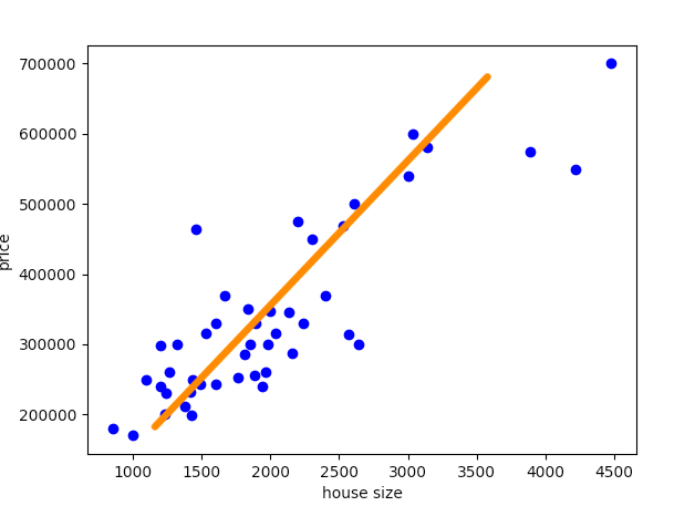
plt.show()调用该函数,将生成下图:
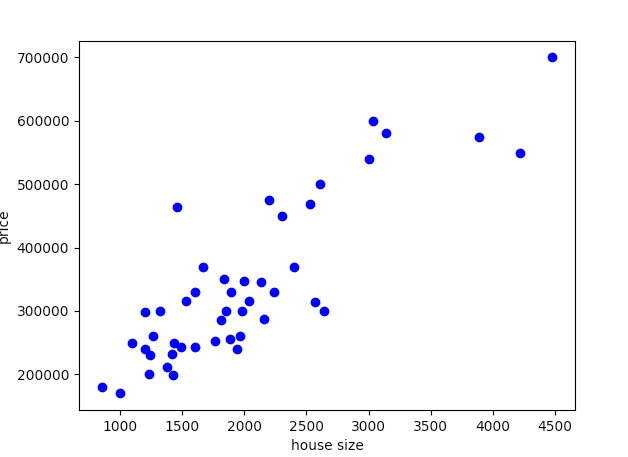
房屋面积与房屋价格关系图。
如上图所示,我们可以粗略地拟合一条线。这意味着使用线性近似能够做出较为准确的预测,因此可以采用线性回归。
准备好数据之后就要进行下一步,给算法编写代码。
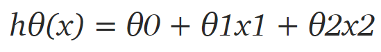
首先我们需要定义假设函数,稍后我们将使用它来计算代价。对于线性回归,假设是:

但数据集中只有 2 个特征,因此对于当前问题,假设是:
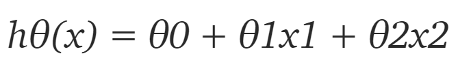
其中 x1 和 x2 是两个特征(即房屋面积和房间数量)。然后编写一个返回该假设的简单 Python 函数:
def h(x,theta):
    return np.matmul(x, theta)
接下来我们来看代价函数。
使用代价函数的目的是评估模型质量。
代价函数的等式为:
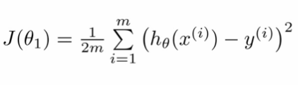
代价函数的代码如下:
def cost_function(x, y, theta):
    return ((h(x, theta)-y).T@(h(x, theta)-y))/(2*y.shape[0])
到目前为止,我们定义的所有 Python 函数都与上述线性回归的数学意义完全相同。接下来我们需要将代价最小化,这就要用到梯度下降。
梯度下降是一种优化算法,旨在调整参数以最小化代价函数。
梯度下降的主要更新步是:
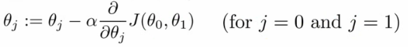
因此,我们将代价函数的导数乘以学习率(α),然后用参数(θ)的当前值减去它,获得新的更新参数(θ)。
def gradient_descent(x, y, theta, learning_rate=0.1, num_epochs=10):
  m = x.shape[0]
  J_all = []

  for _ in range(num_epochs):
    h_x = h(x, theta)
    cost_ = (1/m)*(x.T@(h_x - y))
    theta = theta - (learning_rate)*cost_
    J_all.append(cost_function(x, y, theta))

    return theta, J_all
gradient_descent 函数返回 theta 和 J_all。theta 显然是参数向量,其中包含假设的θs 值,J_all 是一个列表,包含每个 epoch 后的代价函数。J_all 变量并非必不可少,但它有助于更好地分析模型。
接下来要做的就是以正确的顺序调用函数
x,y = load_data("house_price_data.txt")
y = np.reshape(y, (46,1))
x = np.hstack((np.ones((x.shape[0],1)), x))
theta = np.zeros((x.shape[1], 1))
learning_rate = 0.1
num_epochs = 50
theta, J_all = gradient_descent(x, y, theta, learning_rate, num_epochs)
J = cost_function(x, y, theta)
print("Cost: ", J)
print("Parameters: ", theta)

#for testing and plotting cost
n_epochs = []
jplot = []
count = 0
for i in J_all:
  jplot.append(i[0][0])
  n_epochs.append(count)
  count += 1
jplot = np.array(jplot)
n_epochs = np.array(n_epochs)
plot_cost(jplot, n_epochs)

test(theta, [1600, 2])
首先调用 load_data 函数载入 x 和 y 值。x 值包含训练样本,y 值包含标签(在这里就是房屋的价格)。
你肯定注意到了,在整个代码中,我们一直使用矩阵乘法的方式来表达所需。例如为了得到假设,我们必须将每个参数(θ)与每个特征向量(x)相乘。我们可以使用 for 循环,遍历每个样本,每次都执行一次乘法,但如果训练的样本过多,这可能不是最高效的方法。
在这里更有效的方式是使用矩阵乘法。本文所用的数据集具备两个特征:房屋面积和房间数,即我们有(2+1)三个参数。将假设看作图形意义上的一条线,用这种方式来思考额外参数θ0,最终额外的θ0 也要使这条线符合要求。
有利的假设函数图示。
现在我们有了三个参数和两个特征。这意味着θ或参数向量(1 维矩阵)的维数是 (3,1),但特征向量的维度是 (46,2)。你肯定会注意到将这样两个矩阵相乘在数学上是不可能的。再看一遍我们的假设:
如果你仔细观察的话,实际上这很直观:如果在特征向量 (x) {维度为 (46, 3)} 的开头添加额外的一列,并且对 x 和 theta 执行矩阵乘法,将得出 hθ(x) 的方程。
记住,在实际运行代码来实现此功能时,不会像 hθ(x) 那样返回表达式,而是返回该表达式求得的数学值。在上面的代码中,x = np.hstack((np.ones((x.shape[0],1)), x)) 这一行在 x 开头加入了额外一列,以备矩阵乘法需要。
在这之后,我们用零初始化 theta 向量,当然你也可以用一些小随机值来进行初始化。我们还指定了训练学习率和 epoch 数。
定义完所有超参数之后,我们就可以调用梯度下降函数,以返回所有代价函数的历史记录以及参数 theta 的最终向量。在这里 theta 向量定义了最终的假设。你可能注意到,由梯度下降函数返回的 theta 向量的维度为 (3,1)。
还记得函数的假设吗?
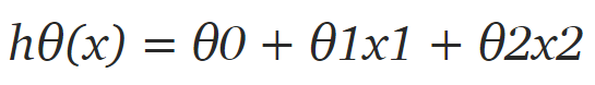
所以我们需要三个θ,theta 向量的维度为 (3,1),因此 theta [0]、theta [1] 和 theta [2] 实际上分别为θ0、θ1 和 θ2。J_all 变量是所有代价函数的历史记录。你可以打印出 J_all 数组,来查看代价函数在梯度下降的每个 epoch 中逐渐减小的过程。
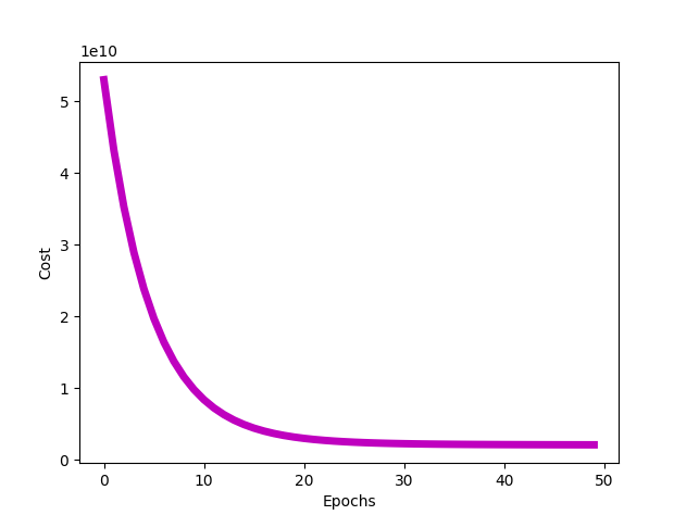
代价和 epoch 数量的关系图。
我们可以通过定义和调用 plot_cost 函数来绘制此图,如下所示:
def plot_cost(J_all, num_epochs):
  plt.xlabel('Epochs')
  plt.ylabel('Cost')
  plt.plot(num_epochs, J_all, 'm', linewidth = "5")
    plt.show()
现在我们可以使用这些参数来找到标签,例如给定房屋面积和房间数量时的房屋价格。
现在你可以测试调用测试函数的代码,该函数会将房屋面积、房间数量和 logistic 回归模型返回的最终 theta 向量作为输入,并输出房屋价格。
def test(theta, x):
  x[0] = (x[0] - mu[0])/std[0]
  x[1] = (x[1] - mu[1])/std[1]

  y = theta[0] + theta[1]*x[0] + theta[2]*x[1]
print("Price of house: ", y)import numpy as np
import matplotlib.pyplot as plt
import pandas as pd
#variables to store mean and standard deviation for each feature
mu = []
std = []
def load_data(filename):
df = pd.read_csv(filename, sep=",", index_col=False)
df.columns = ["housesize", "rooms", "price"]
data = np.array(df, dtype=float)
plot_data(data[:,:2], data[:, -1])
normalize(data)
return data[:,:2], data[:, -1]
def plot_data(x, y):
plt.xlabel('house size')
plt.ylabel('price')
plt.plot(x[:,0], y, 'bo')
plt.show()
def normalize(data):
for i in range(0,data.shape[1]-1):
data[:,i] = ((data[:,i] - np.mean(data[:,i]))/np.std(data[:, i]))
mu.append(np.mean(data[:,i]))
std.append(np.std(data[:, i]))
def h(x,theta):
return np.matmul(x, theta)
def cost_function(x, y, theta):
return ((h(x, theta)-y).T@(h(x, theta)-y))/(2*y.shape[0])
def gradient_descent(x, y, theta, learning_rate=0.1, num_epochs=10):
m = x.shape[0]
J_all = []
for _ in range(num_epochs):
h_x = h(x, theta)
cost_ = (1/m)*(x.T@(h_x - y))
theta = theta - (learning_rate)*cost_
J_all.append(cost_function(x, y, theta))
return theta, J_all
def plot_cost(J_all, num_epochs):
plt.xlabel('Epochs')
plt.ylabel('Cost')
plt.plot(num_epochs, J_all, 'm', linewidth = "5")
plt.show()
def test(theta, x):
x[0] = (x[0] - mu[0])/std[0]
x[1] = (x[1] - mu[1])/std[1]
y = theta[0] + theta[1]*x[0] + theta[2]*x[1]
print("Price of house: ", y)
x,y = load_data("house_price_data.txt")
y = np.reshape(y, (46,1))
x = np.hstack((np.ones((x.shape[0],1)), x))
theta = np.zeros((x.shape[1], 1))
learning_rate = 0.1
num_epochs = 50
theta, J_all = gradient_descent(x, y, theta, learning_rate, num_epochs)
J = cost_function(x, y, theta)
print("Cost: ", J)
print("Parameters: ", theta)
#for testing and plotting cost
n_epochs = []
jplot = []
count = 0
for i in J_all:
jplot.append(i[0][0])
n_epochs.append(count)
count += 1
jplot = np.array(jplot)
n_epochs = np.array(n_epochs)
plot_cost(jplot, n_epochs)
test(theta, [1600, 3])上述就是小编为大家分享的使用Python怎么书写一个线性回归了,如果刚好有类似的疑惑,不妨参照上述分析进行理解。如果想知道更多相关知识,欢迎关注亿速云行业资讯频道。
免责声明:本站发布的内容(图片、视频和文字)以原创、转载和分享为主,文章观点不代表本网站立场,如果涉及侵权请联系站长邮箱:is@yisu.com进行举报,并提供相关证据,一经查实,将立刻删除涉嫌侵权内容。


